In the last part of this series, we learned how to simulate a point mass making frictional contact with the ground plane.
This time, we’ll do the same thing, but with a three-dimensional cube.
Modeling a Floating Rigid Body
Let’s start by making our cube float in a zero-G environment.
Dynamics
To simulate a three-dimensional rigid body, our new state-space system must encapsulate not just the object’s position and linear velocity, but also its orientation/attitude and angular velocity. That leads us to the following state vector:
$$ \begin{equation} \boldsymbol{X} = \begin{bmatrix} \boldsymbol{r_W} \\ \boldsymbol{q} \\ \boldsymbol{v_W} \\ \boldsymbol{\omega_B} \end{bmatrix} \end{equation} $$Where:
- $\boldsymbol{r_W}$ is the body’s world-frame position.
- $\boldsymbol{q}$ is the body’s attitude quaternion (representing a rotation from the body frame to the world frame).
- $\boldsymbol{v_W}$ is the body’s world-frame linear velocity.
- $\boldsymbol{\omega_B}$ is the body-frame angular velocity.
As before, we need to formulate the state vector’s derivative $\boldsymbol{\dot{X}}$ in order to time-step. This starts out easy: the derivative of $\boldsymbol{r_W}$ is just $\boldsymbol{v_W}$.
Differentiating the attitude quaternion is a bit trickier; it requires the following transformation to be applied, where $\otimes$ represents a quaternion multiplication operation. I won’t get into the derivation of that here because that could take up an entire blog post by itself. If you’re curious, look to section 4.5 of 1.
$$ \begin{equation} \boldsymbol{\dot{q}} = \frac{1}{2} \boldsymbol{q} \otimes \begin{bmatrix} 0 \\ \boldsymbol{\omega_B} \\ \end{bmatrix} \end{equation} $$For convenience, we can express the quaternion multiplication operation as a matrix operation, using $L(\boldsymbol{q})$ as defined in 2 and 3. We can also use $H$ as follows to reshape $\boldsymbol{\omega_B}$.
For the derivatives of linear and angular velocity, we need to consider the effect of external forces $\boldsymbol{f_W}$ and torques $\boldsymbol{\tau_B}$ on the body. Equation (5) is just $f = ma$. Equation (6) is Euler’s rotation equation, where $I$ is the inertia matrix.
$$ \begin{equation} \boldsymbol{f_W} = m \boldsymbol{\dot{v}_W} \end{equation} $$ $$ \begin{equation} \boldsymbol{\tau_B} = I \boldsymbol{\dot{\omega}_B} + \boldsymbol{\omega_B} \times I \boldsymbol{\omega_B} \end{equation} $$Putting all of that together, we get the following nonlinear system.
$$ \begin{equation} \boldsymbol{\dot{X}} = \begin{bmatrix} \boldsymbol{\dot{r}_W} \\ \boldsymbol{\dot{q}} \\ \boldsymbol{\dot{v}_W} \\ \boldsymbol{\dot{\omega}_B} \end{bmatrix} = \begin{bmatrix} \boldsymbol{v_W} \\ \frac{1}{2}L(\boldsymbol{q})H\boldsymbol{\omega_B} \\ \frac{1}{m}\boldsymbol{f_W} \\ I^{-1}(\boldsymbol{\tau_B} + \boldsymbol{\omega_B} \times I \boldsymbol{\omega_B}) \\ \end{bmatrix} \end{equation} $$Kinematics
To visualize the cube, and to simulate contact later, we’ll need to solve for the world-frame position of every corner of the cube.
First, we’ll define $C_B \in \mathbb{R}^{8 \times 3}$, a matrix containing the cube’s eight body-frame corner positions. (I have chosen the cube’s dimensions somewhat arbitrarily.)
We’ll also need to convert the attitude quaternion $\boldsymbol{q}$ into $A$, its rotation matrix equivalent.
Then we can solve for the matrix of world-frame corner positions, $C_W\in \mathbb{R}^{8 \times 3}$, as follows.
Now let’s look at the Python code.
The Code
We’ll start with imports, including necessary quaternion operations.
from collections.abc import Callable

import numpy as np
import pyvista as pv
from tqdm import tqdm

import plotting
from transforms import Aq, H, Lq
Then we’ll define the timestep size, mass, and inertia matrix as global variables.
# mass of the particle in kg
MASS = 10
# inertia matrix
INERTIA = np.eye(3) * 0.01
# inertia matrix inverse
I_INV = np.linalg.inv(INERTIA)
# timestep size
DT = 0.001
We’ll also define $C_B$ and the kinematics function that returns $C_W$ here.
C_B = np.array(
    (
        [-1, -1, -1],
        [1, -1, -1],
        [-1, 1, -1],
        [1, 1, -1],
        [-1, -1, 1],
        [1, -1, 1],
        [-1, 1, 1],
        [1, 1, 1],
    )
)

def kin_corners(X: np.ndarray) -> np.ndarray:
    ones_nc = np.ones((8, 1))
    # position of cube in world frame
    r_w = X[0:3].reshape((-1, 1))
    # body to world frame quaternion
    Q = X[3:7]
    # rotation matrix
    A = Aq(Q)
    # rotate C_B and add r_w
    C_W = (A @ C_B.T).T + ones_nc @ r_w.T
    return C_W
Next, we’ll define the continuous-time dynamics from Equation (7).
def dynamics_floating_ct(X: np.ndarray, U: np.ndarray) -> np.ndarray:
    """
    Continuous-time SE(3) nonlinear dynamics

    :param X: state vector
    :param U: control vector
    """
    Q = X[3:7]  # B to W
    v_w = X[7:10]  # W frame
    ω_b = X[10:13]  # B frame
    F_w = U[0:3]  # W frame
    tau_b = U[3:]  # B frame
    dr = v_w
    dq = 0.5 * Lq(Q) @ H @ ω_b
    dv = 1 / MASS * F_w
    dω = I_INV @ (tau_b - np.cross(ω_b, INERTIA @ ω_b))
    dX = np.hstack((dr, dq, dv, dω)).T
    return dX
We’ll also write a function to perform RK4 integration. It’s similar to the one introduced in Part 1 of this series, except that there’s an extra step to prevent quaternion drift.
def rk4_normalized(dynamics: Callable, X_k: np.ndarray, U_k: np.ndarray) -> np.ndarray:
    """
    RK4 integrator

    :param dynamics: dynamics function
    :param X_k: state vector at step k
    :param U_k: control vector at step k
    """
    f1 = dynamics(X_k, U_k)
    f2 = dynamics(X_k + 0.5 * DT * f1, U_k)
    f3 = dynamics(X_k + 0.5 * DT * f2, U_k)
    f4 = dynamics(X_k + DT * f3, U_k)
    xn = X_k + (DT / 6.0) * (f1 + 2 * f2 + 2 * f3 + f4)
    # normalize the quaternion term
    xn[3:7] = xn[3:7] / np.linalg.norm(xn[3:7])
    return xn
Finally, we’ll create a function that uses PyVista to animate the cube given its state history and the kinematics function from earlier.
def animate_cube(X_hist: np.ndarray, dt: float, name: str) -> None:
    """
    Convert state hist into gif

    :param X_hist: state history
    :param dt: timestep size
    :param name: filename
    """
    N = np.shape(X_hist)[0]
    mesh = pv.Box()
    mesh_plane = pv.Plane(i_size=20, j_size=20, i_resolution=1, j_resolution=1)
    text_obj = pv.Text("t = 0.00 s", position=[0, 0])
    text_obj.prop.color = "black"
    text_obj.prop.font_size = 20
    plotter = pv.Plotter(notebook=False, off_screen=True, window_size=[800, 800])
    plotter.add_mesh(mesh, show_edges=True, color="white")
    plotter.add_mesh(mesh_plane, show_edges=True, color="white")
    plotter.camera.zoom(1.5)
    plotter.add_actor(text_obj)
    fps = 30.0
    speed = 1  # x real time
    plotter.open_gif(
        "results/" + name + ".gif", fps=fps, palettesize=64, subrectangles=True
    )
    # steps/frame = s/frame * steps/s = 1 / (((frames/s) * (s/step))
    steps_per_frame = int(speed / (fps * dt))
    for k in tqdm(range(N)[::steps_per_frame], desc="Generating gif"):
        r_c = kin_corners(X_hist[k, :])
        text_obj.input = "t = " + f"{round(k * dt, 2):.2f}" + "s"
        mesh.points = r_c
        plotter.write_frame()

    # Closes and finalizes movie
    plotter.close()
The rest is quite simple.
We initialize with an arbitrary starting state and integrate through the dynamics in a for loop. At the end, we use animate_cube to visualize the result.
def main():
    N = 1200  # number of timesteps
    n_x = 13  # length of state vector
    n_u = 6  # length of control vector

    # initialize starting state
    X_0 = np.zeros(n_x)
    # position
    X_0[:3] = np.array([0, 0, 3.0])
    # quaternion
    X_0[3:7] = np.array([1, 0, 0, 0])
    # linear velocity
    X_0[7:10] = np.array([2, 0, 0])
    # angular velocity
    X_0[10:13] = np.array([2.0, 4.0, 6.0])

    # array of state vectors for each timestep
    X_hist = np.zeros((N, n_x))
    X_hist[0, :] = X_0
    # array of control vectors for each timestep
    U_hist = np.zeros((N - 1, n_u))

    for k in range(N - 1):
        X_hist[k + 1, :] = rk4_normalized(
            dynamics_floating_ct, X_hist[k, :], U_hist[k, :]
        )

    name = "cube_3d_floating"
    animate_cube(X_hist, DT, name)
The full code for this demonstration can be found here.
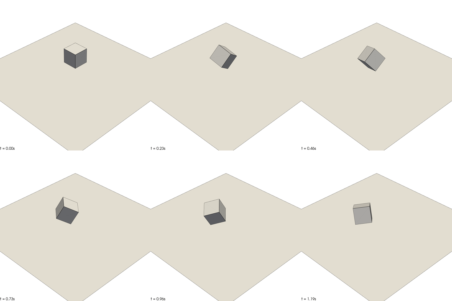
Here’s the result. As expected, we see the cube drifting through space with constant linear and angular velocities.
Rigid Body Contact and Friction
Now for the hard part: implementing contact and friction. We’ll start with the optimization problem and work backward from there.
The Optimization Problem
The optimization problem, solved per timestep, is as follows.
$$ \begin{align} \min_{\boldsymbol{X}_{k+1}, \boldsymbol{F}_k, \boldsymbol{s_1}, \boldsymbol{s_2}, \boldsymbol{\lambda}} \quad & \boldsymbol{s_1}^\intercal \boldsymbol{s_1} + \boldsymbol{s_2}^\intercal \boldsymbol{s_2} \\ \textrm{s.t.} \quad & \bold{f}(\boldsymbol{X}_k, \boldsymbol{F}_k, \boldsymbol{X}_{k+1}) - \boldsymbol{X}_{k+1} = 0 \\ & ||\boldsymbol{q}_{k+1}||^2 - 1 = 0 \\ & s_{1, i} - f_{z, i} z_{k+1, i} \geq 0 \quad &&\forall i \in \{1, \dots, 8\}\\ & \alpha_i \left(\boldsymbol{c}_{xy, i} + \lambda_i \frac{\boldsymbol{f}_{xy, i}}{||\boldsymbol{f}_{xy, i}||_\epsilon + \epsilon}\right) = 0 \quad &&\forall i \in \{1, \dots, 8\}\\ & \mu f_{z, i} - ||\boldsymbol{f}_{xy, i}||_\epsilon \geq 0 \quad &&\forall i \in \{1, \dots, 8\}\\ & s_{2, i} - \lambda_i (\mu f_{z, i} - ||\boldsymbol{f}_{xy, i}||_\epsilon) \geq 0 \quad &&\forall i \in \{1, \dots, 8\}\\ & z_{k+1}, f_z, \boldsymbol{s_1}, \boldsymbol{s_2}, \boldsymbol{\lambda} \geq 0 \\ \end{align} $$Where:
- $\bold{f}(X_k, \boldsymbol{F}_k, \boldsymbol{X}_{k+1})$ represents the system’s discrete-time dynamics.
- The variable $\boldsymbol{F}_k \in \mathbb{R}^{8 \times 3}$ is a matrix of world-frame contact forces per timestep $k$, where each row $\boldsymbol{f}_i \in \mathbb{R}^3$ represents the force acting on corner $i \in \set{1, \dots, 8}$ of the cube. Force vector $\boldsymbol{f}_i$ is further partitioned into its planar tangential and normal components $\boldsymbol{f}_{xy, i} \in \mathbb{R}^2$ and $f_{z, i} \in \mathbb{R}$, respectively. (This partitioning gets more complex if the ground isn’t flat, but here we’ll assume that it is).
- Variables $\boldsymbol{s_1}$, $\boldsymbol{s_2}$, and $\boldsymbol{\lambda}$ are also now vectors $\in \mathbb{R}^8$ and taken per timestep $k$.
- Variable $\boldsymbol{z}_{k+1} \in \mathbb{R}^8$ is a vector of corner heights at timestep $k+1$. This variable is extracted from $C_{W, k+1}$.
- Variable $\boldsymbol{c}_{xy, i} \in \mathbb{R}^{2}$ is the tangential velocity of corner $i$ at timestep $k$.
- Variable $\alpha_i \in \lbrace0, 1 \rbrace$ flags whether or not corner $i$ is in contact. More on this later.
- Eq. (13) enforces quaternion normalization.
- Eq. (14), the interpenetration complementarity constraint, keeps z-axis forces at zero when contact is not being made.
- Eq. (15), the maximum dissipation constraint, constrains the tangential velocity lagrange multiplier $\lambda_i$ to $\boldsymbol{c}_{xy, i}$ and enforces the direction of the friction force vector.
- Eq. (16), the friction cone constraint, enforces the relationship between normal force, friction coefficient, and frictional force.
- Eq. (17), the friction complementarity constraint, drives friction forces to zero when tangential velocity is zero.
While at first glance this doesn’t look too different from the previous post, there are still several missing pieces to this puzzle.
Handling Multi-Contact Dynamics
The system’s discrete-time dynamics can be calculated by integrating the continuous-time dynamics from Eq. (7). However, to use Eq. (7) we will need to convert the $\boldsymbol{F}_k \in \mathbb{R}^{8 \times 3}$ from our optimization problem into $\boldsymbol{f_W}\in \mathbb{R}^{3}$ and $\boldsymbol{\tau_B}\in \mathbb{R}^{3}$.
The conversion for $\boldsymbol{f_W}$ is quite simple: it’s just a row-wise summation of $\boldsymbol{F}_k$. In matrix math, it can be done as shown below. Note that $\boldsymbol{1_8}$ is an $8 \times 1$ vector of ones.
The conversion for $\boldsymbol{\tau_B}$ is as follows, where $\boldsymbol{c}_i$ and $\boldsymbol{f}_i$ are slices of $C_B$ and $\boldsymbol{F}_k$ per corner.
Solving for Tangential Velocity
The tangential velocity variable can’t be extracted directly from $\boldsymbol{X}_k$ like it was last time. Instead, we’ll have to solve for $C_{W, k}$ and $C_{W, k+1}$ using Eq. (10).
Then we can approximate the corner velocities matrix, $\dot{C}\in \mathbb{R}^{8 \times 3}$.
Velocity variable $\boldsymbol{c}_{xy, i} \in \mathbb{R}^{2}$ is just the tangential partition of $\dot{C}$ at corner $i$.
Flagging Contact
You may be wondering why the maximum dissipation constraint (Eq. (15)) now has the additional variable $\alpha_i$. Well, let’s think about this for a second.
Given the following equation, what happens when the cube is mid-air and has a nonzero tangential velocity?
Since $\boldsymbol{\dot{c}}_{xy, i}$ is nonzero, the righthand term must also be nonzero. Which means that $\boldsymbol{f}_{xy, i}$ is nonzero, even though the cube is not in contact with the ground. So this actually shouldn’t work.
In fact, it only worked in the previous chapter because the solver allowed the tangential force to be slightly above zero, and jacked up $\boldsymbol{\lambda}$ until the equation was satisfied. In the 3D case, the optimization problem is too complex and nonlinear for this cheat to work.
Logically, the constraint could be rectified as follows.
This way, the constraint is automatically turned off when contact is not being made. This method is proposed in 4. However, there is a catch in our implementation: as an interior-point optimizer, IPOPT does not allow variables to touch their absolute limits. Therefore, in the absence of contact, $f_{z, i}$ would be infinitesimal rather than exactly zero, which ruins the whole thing.
The workaround is to clamp the upper and lower bounds of $f_{z, i}$ to zero whenever contact isn’t detected. This actually does work.
But now you’re explicitly checking for contact per timestep outside of the solver! So if you’re already doing that, why not use the contact flag itself to activate/deactivate the constraint? I compared the two strategies, and found that using the contact flag in Eq. (15) results in about double the solve speed and less instability. This is probably because it makes the optimization problem simpler. It’s basically spoon-feeding contact to the solver.
The Code
We start with imports, as always. This time we’re importing a bunch of useful stuff from the floating version of the code above.
from collections.abc import Callable

import casadi as cs
import numpy as np
from tqdm import tqdm

import plotting
from cube_3d_floating import (
    C_B,
    I_INV,
    INERTIA,
    MASS,
    animate_cube,
    kin_corners,
)
from error_suppression import suppress_stderr
from transforms_cs import Aq_cs, H, Lq_cs
Then we define the timestep size, gravitational constant, and coefficient of friction $\mu$, as well as the solver tolerance and the smoothnorm function from the previous chapter.
# timestep size
DT = 0.002
# gravity
G = 9.81
# coefficient of friction
MU = 0.3
# solver tolerance
ϵ = 1e-6


def smoothnorm(x: cs.SX):
    return cs.sqrt(x.T @ x + ϵ * ϵ) - ϵ
We will also need to create a modified version of the kinematics function from earlier that is adapted to CaSaDi’s datatypes rather than numpy’s.
def kin_corners_cs(X: cs.SX) -> cs.SX:
    r_c = cs.SX(8, 3)
    ones_nc = cs.SX.ones(8, 1)
    r_w = X[0:3]  # W frame
    Q = X[3:7]  # B to W
    A = Aq_cs(Q)  # rotation matrix
    r_c = C_B @ A.T + ones_nc @ r_w.T
    return r_c
Next, we create a modified version of the dynamics function that includes the conversion of $\boldsymbol{F}_k$ into $\boldsymbol{f_W}$ and $\boldsymbol{\tau_B}$ from Eqs. (19) and (20). Gravity is also applied as a force.
def dynamics_confr_ct(X: cs.SX, F: cs.SX) -> cs.SX:
    """
    Continuous-time SE(3) nonlinear dynamics
    Subject to gravity and 3D collision forces

    :param X: state vector
    :param F: forces (8x3), vector per corner
    """
    Q = X[3:7]  # B to W
    v_w = X[7:10]  # W frame
    ω_b = X[10:13]  # B frame

    # rotation matrix, body to world frame
    A = Aq_cs(Q)

    # get sum of all forces in world frame
    # 3x1 = 3x8 @ 8x1
    ones_nc = cs.SX.ones(8, 1)
    F_w = F.T @ ones_nc  # force in W frame
    tau_b = cs.SX(3, 1)  # torque in B frame
    for i in range(8):
        # add body frame torque due to body frame force
        tau_b += cs.cross(C_B[i, :], A.T @ F[i, :].T)

    # apply gravity
    F_w += np.array([0, 0, -G]) * MASS

    dr = v_w
    dq = 0.5 * Lq_cs(Q) @ H @ ω_b
    dv = 1 / MASS * F_w
    dω = I_INV @ (tau_b - cs.cross(ω_b, INERTIA @ ω_b))
    dX = cs.vertcat(dr, dq, dv, dω)
    return dX
We will also want to define a semi-implicit Euler integrator for the above dynamics. As mentioned in Part 2, it plays better with the optimizer than RK4.
def euler_semi_implicit(
    dynamics: Callable,
    X_k: cs.SX,
    U_k: cs.SX,
    X_k1: cs.SX,
) -> cs.SX:
    """
    Semi-Implicit Euler Integrator

    :param dynamics: dynamics function
    :param X_k: state vector at step k
    :param U_k: control vector at step k
    :param X_k1: state vector at step k+1
    """
    X_k_semi = cs.SX.zeros(13)
    X_k_semi[:7] = X_k[:7]
    X_k_semi[7:] = X_k1[7:]
    X_n = X_k + DT * dynamics(X_k_semi, U_k)
    # normalize the quaternion term
    X_n[3:7] = X_n[3:7] / cs.norm_2(X_n[3:7])
    return X_n
Let us now initialize our CaSaDi variables and define the objective:
def main():
    n_a = 13  # length of state vector
    n_c = 8  # number of contact points on cube
    # initialize casadi variables
    Xk1 = cs.SX.sym("Xk1", n_a)  # X(k+1), state at next timestep
    F = cs.SX.sym("F", n_c, 3)  # force vector at each corner
    s1 = cs.SX.sym("s1", n_c)  # slack variable 1
    s2 = cs.SX.sym("s2", n_c)  # slack variable 2
    # lagrange mult for magnitude of ground vel per contact point
    lam = cs.SX.sym("lam", n_c)
    X = cs.SX.sym("X", n_a)  # X(k), state
    alpha = cs.SX.sym("con", n_c)  # contact flags, 8x1

    C_prev = kin_corners_cs(X)  # corner positions at k, 8x3
    C = kin_corners_cs(Xk1)  # corner positions at k+1, 8x3
    dC_xy = ((C - C_prev) / DT)[:, 0:2]  # corner xy velocities, 8x2
    c_z = C[:, 2]  # corner heights at k+1, 8x1
    F_xy = F[:, :2]  # tangential ground force friction vectors, 8x2
    F_z = F[:, 2]  # vertical grfs, 8x1

    # objective
    obj = s1.T @ s1 + s2.T @ s2
Next, we’ll define the constraints:
constr = []  # init constraints

    # --- Equality Constraints --- #
    constr = cs.vertcat(constr, euler_semi_implicit(dynamics_confr_ct, X, F, Xk1) - Xk1)

    # quaternion normalization
    constr = cs.vertcat(constr, cs.norm_2(Xk1[3:7]) ** 2 - 1)

    # max dissipation for each corner (relaxed in air)
    for i in range(n_c):
        constr = cs.vertcat(
            constr,
            alpha[i]
            * (dC_xy[i, :].T + lam[i] * F_xy[i, :].T / (smoothnorm(F_xy[i, :].T) + ϵ)),
        )

    # --- Inequality Constraints --- #
    # interpenetration
    constr = cs.vertcat(constr, c_z)

    # primal feasibility friction cone
    for i in range(n_c):
        constr = cs.vertcat(constr, MU * F_z[i] - smoothnorm(F_xy[i, :].T))

    # interpenetration complementarity
    constr = cs.vertcat(constr, s1 - F_z * c_z)

    # friction complementarity
    for i in range(n_c):
        constr = cs.vertcat(
            constr, s2[i] - lam[i] * (MU * F_z[i] - smoothnorm(F_xy[i, :].T))
        )
Next, we build the optimization problem.
    opt_variables = cs.vertcat(Xk1, F[:, 0], F[:, 1], F[:, 2], s1, s2, lam)
    parameters = cs.vertcat(X, alpha)
    lcp = {"x": opt_variables, "p": parameters, "f": obj, "g": constr}
    opts = {
        "print_time": 0,
        "ipopt.print_level": 0,
        "ipopt.sb": "yes",  # Silences the IPOPT startup banner
        "ipopt.tol": ϵ,
        "ipopt.max_iter": 300,
    }

    solver = cs.nlpsol("S", "ipopt", lcp, opts)
Then we define variable and constraint bounds.
    n_var = np.shape(opt_variables)[0]
    n_g = np.shape(constr)[0]

    # variable bounds
    ubx = [1e10] * n_var
    lbx = [0] * n_var
    lbx[:n_a] = [-1e10] * n_a  # state can be negative
    lbx[n_a : n_a + n_c * 2] = [-1e10] * (n_c * 2)  # Fx and Fy can be negative

    # constraint bounds
    ubg = [0] * n_g
    ubg[n_a + 1 + n_c * 2 :] = [1e10] * (n_c * 4)  # inequality constraints
    lbg = [0] * n_g
Next, we initialize the simulation variables.
    N = 1000  # number of timesteps
    X_0 = np.zeros(n_a)
    X_0[:3] = np.array([0, 0, 2.5])
    X_0[3:7] = np.random.rand(4)
    X_0[3:7] = X_0[3:7] / np.linalg.norm(X_0[3:7])  # normalize the quaternion
    X_0[7:10] = np.array([0, 4, 0])
    X_0[10:13] = np.array([0, -2, 1])

    X_hist = np.zeros((N, n_a))  # state vector for each timestep
    Fx_hist = np.zeros((N, n_c))  # array of corner Fx for each timestep
    Fy_hist = np.zeros((N, n_c))  # array of corner Fy for each timestep
    Fz_hist = np.zeros((N, n_c))  # array of corner Fz for each timestep
    s1_hist = np.zeros((N, n_c))  # array of slack var 1 values for each timestep
    s2_hist = np.zeros((N, n_c))  # array of slack var 2 values for each timestep
    lam_hist = np.zeros((N, n_c))  # array of lambda values for each timestep

    prev_sol = np.hstack((X_0, np.zeros(n_c * 6)))
    X_hist[0, :] = X_0
Finally, we can loop through the timesteps.
Notice how we’re explicitly checking for contact and then feeding that into the solver.
The set of contact flags $\alpha$ becomes a solver parameter that updates the optimization problem per timestep.
We also explicitly clamp the forces, slack variables, and $\boldsymbol{\lambda}$ to zero for corners that aren’t in contact.
This makes the optimization problem appear to be overconstrained, causing CaSaDi to spit out a lot of warnings.
But these warnings can be ignored, because IPOPT automatically detects the equality constraints and treats them as fixed variables.
The suppress_stderr() function silences CaSaDi’s warnings.
    for k in tqdm(range(N - 1), desc="Simulating"):
        # get corner heights
        c_z_k = kin_corners(X_hist[k, :])[:, 2]
        # check which corners are in contact
        alpha_k = (c_z_k <= 0.005).astype(float)
        # update parameter values for contact
        parameter_values = np.hstack((X_hist[k, :], alpha_k))
        ubx_k = ubx.copy()
        lbx_k = lbx.copy()
        for i in range(n_c):
            if alpha_k[i] == 0.0:
                # no contact at this corner, set forces to zero
                ubx_k[n_a + i] = 0.0  # fx upper
                lbx_k[n_a + i] = 0.0  # fx lower
                ubx_k[n_a + n_c + i] = 0.0  # fy upper
                lbx_k[n_a + n_c + i] = 0.0  # fy lower
                ubx_k[n_a + n_c * 2 + i] = 0.0  # fz upper
                lbx_k[n_a + n_c * 2 + i] = 0.0  # fz lower
                # clamp slack variables and lambda
                ubx_k[n_a + n_c * 3 + i] = 0.0  # s1
                ubx_k[n_a + n_c * 4 + i] = 0.0  # s2
                ubx_k[n_a + n_c * 5 + i] = 0.0  # lam

        with suppress_stderr():
            sol = solver(
                x0=prev_sol, lbx=lbx_k, ubx=ubx_k, lbg=lbg, ubg=ubg, p=parameter_values
            )
        X_hist[k + 1, :] = np.reshape(sol["x"][0:n_a], (-1,))
        Fx_hist[k] = np.reshape(sol["x"][n_a : n_a + n_c], (-1,))
        Fy_hist[k] = np.reshape(sol["x"][n_a + n_c : n_a + n_c * 2], (-1,))
        Fz_hist[k] = np.reshape(sol["x"][n_a + n_c * 2 : n_a + n_c * 3], (-1,))
        s1_hist[k] = np.reshape(sol["x"][n_a + n_c * 3 : n_a + n_c * 4], (-1,))
        s2_hist[k] = np.reshape(sol["x"][n_a + n_c * 4 : n_a + n_c * 5], (-1,))
        lam_hist[k] = np.reshape(sol["x"][n_a + n_c * 5 :], (-1,))
        prev_sol = sol["x"]  # sol

    name = "cube_3d_confr_tstep"
    hists = {
        "x (m)": X_hist[:, 0],
        "y (m)": X_hist[:, 1],
        "z (m)": X_hist[:, 2],
        "Fz (N)": Fz_hist,
        "s1": s1_hist,
        "s2": s2_hist,
        "lam": lam_hist,
    }
    plotting.plot_hist(hists, name)
    animate_cube(X_hist, DT, name)
The full code can be found here.
Here’s the result!
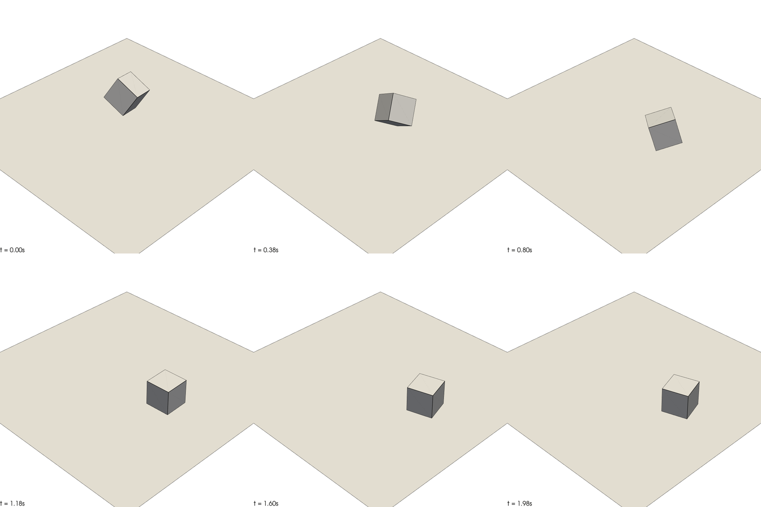
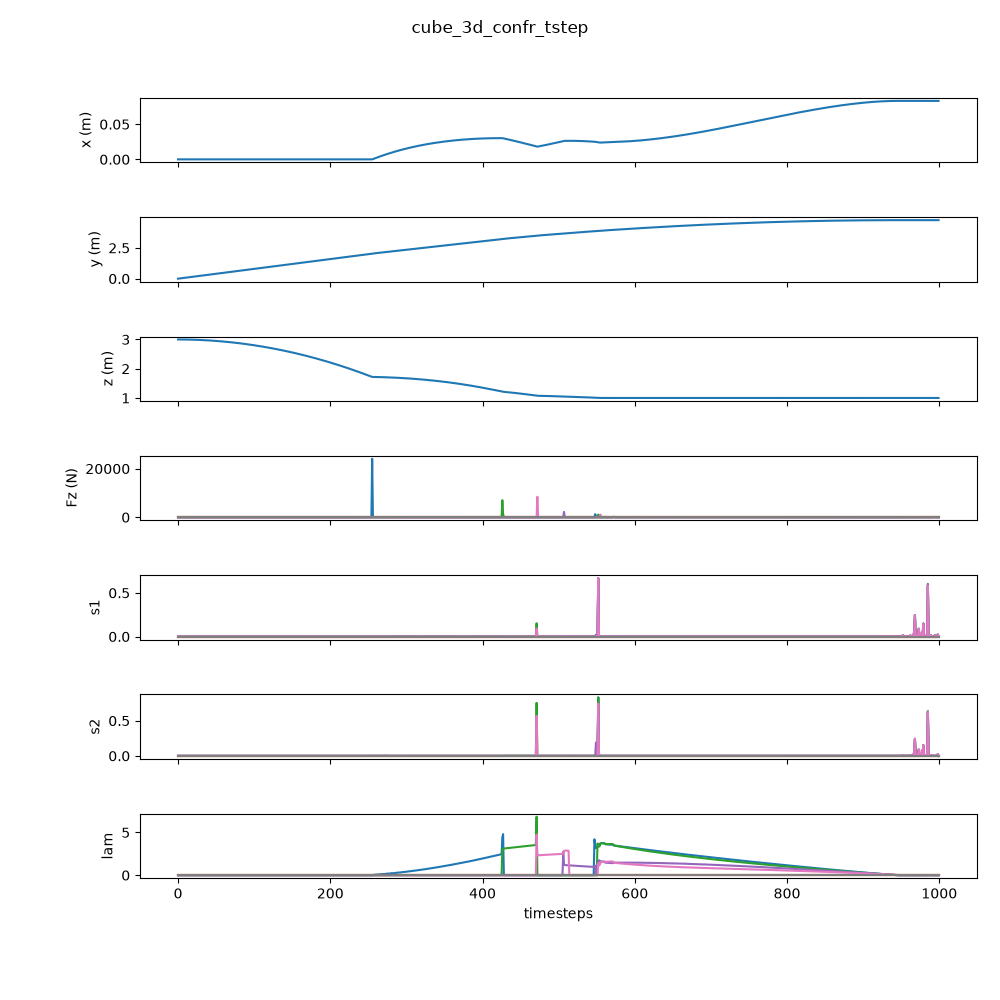
Simulation speed is pretty inconsistent depending on the randomized starting quaternion, because solve time per timestep is dependent on how many points are in contact and how fast they’re moving. This particular run took about thirty seconds to solve on my Framework 13, but with the right custom solver it should easily be doable in real time or faster. That’s way outside of the scope of this post, though.
References
J. Sola, “Quaternion kinematics for the error-state Kalman filter,” arXiv preprint arXiv:1711.02508, 2017. ↩︎
B. E Jackson, K. Tracy, and Z. Manchester, “Planning with attitude,” IEEE Robotics and Automation Letters, vol. 6, no. 3, pp. 5658–5664, 2021. ↩︎
N. Trawny and S. I. Roumeliotis, “Indirect Kalman filter for 3D attitude estimation,” University of Minnesota, Dept. of Comp. Sci. & Eng., Tech. Rep, vol. 2, p. 2005, 2005. ↩︎
M. Posa, C. Cantu, and R. Tedrake, “A direct method for trajectory optimization of rigid bodies through contact,” The International Journal of Robotics Research, vol. 33, no. 1, pp. 69–81, 2014. ↩︎